EMere 2.6 | Heat Conduction!

The time has finally come! Multiphysics is coming to EMerge.

Soon, EMerge version 2.6 will be released which includes the first version of the heat conduction solver. It also allows for one-way RF-to-heat conduction coupling.

Heat conduction involves only the conduction of heat through materials. It does not include the simulation of fluid flow which is a dominant form of heat transport in for example convection cooling such as with computer fans.

None-the-less approximate convection figures can be used to still get good estimations for thermal conduction.

In this blog post I will demonstrate the capabilities of the heat conduction solver in EMerge based on the new heat conduction example files:

• demo1_basic_simulation.py

• demo2_chip_heating.py

• demo3_RF_heating.py

• demo4_black_body_radiation.py

• demo5_transient_heat_conduction.py

NLnet funding

I am very happy to be able to say that the development of the thermal solver is funded by NLnet. You can read more about NLnet here: https://nlnet.nl/project/EMerge/

Whats included?

The heat conduction module has a lot of the important features! There are still some holes remaining that are to be plugged. But first, lets summarize briefliy what has been added:

Boundary Conditions

1. Fixed Temperature

2. Heat flux (heat injection in W/m² or W/m³)

3. Initial temperature (for transient solvers)

4. Convection (heat flow to ambient through finite conductivity)

5. Thermal Contact (Heat flux resistance at boundary interface)

6. Thin Conductor (heat distribution through 2D conducting surfaces)

7. Black body radiation (non-linear)

Solvers

1. Steady state solver

2. Transient solver (linear)

   1. Backwards Euler

   2. Crank-Nicolson

3. Non-linear Steady state solver with Anderson Acceleration

4. Cholesky solver interface through scikit-sparse (optional dependency)

5. Iterative solver with block-Jacobi pre-conditioner

Multi-physics

1. Volumetric heat flux from volumetric dissipation

2. One-way coupling (RF losses -> Thermal simulation)

Demo 1: Heat conduction in a metal rod

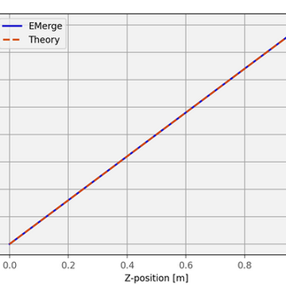
The first demo is just a basic simulation of a teflon rod with a fixed temperature on one side and a heat flux on the other side.

What is nice about this thermal problem is that the solution is a really easy analytical constant thermal gradient proportional to the heat flux divided by the thermal conductivity of the material.

Because the solution is simple, these also make for really good validation tests for the test suite.

The temperature profile inside the rod

3D Cloud plot of the temperature relative to ambient

The mesh of the 3D Rod

The Teflon rod geometry

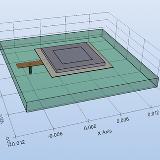
Demo 2: Chip Heating

The second demo is a simplified simulation setup with some dummy parameters of heating in a chip. No simulation of electronics are involved here. The temperature is just modeled as a boundary heat source injecting a total power of 5 Watts into the 5mm x 5mm chip. A thermal interface material (TIM) is placed in between the chip and the PCB. An extra copper trace is added to demonstrate the heat flux through thin conductors.

The mesh of the chip heating module

A 2D slice of showing the temperature and heat flux quiver plot.

The geometry of the chip heating example.

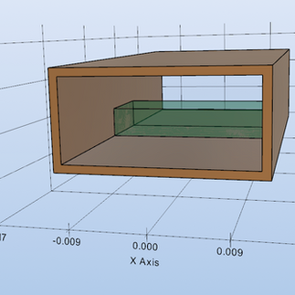
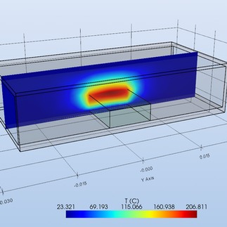
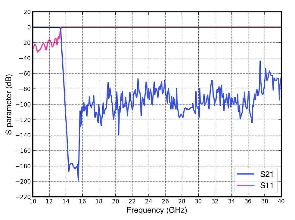
Demo 3: RF heating

In the third demo we look at microwave heating of a dielectric block in a WR90 rectangular waveguide that is exposed by a 100W of power. The waveguide is modeled with a 1mm thick copper wall. The dielectric block is made of FR4 material. The bottom of the waveguide is connected to a thermal ground. The simulation is ran at 10GHz after which the heating is used as a volumetric heat flux source in the Thermal simulation. Just this one line is all that is needed!

The copper waveguide wall with the dielectric FR4 Block inside

The model mesh

The Ez-field animation with a cloud plot showing the volumetric heat generation.

The temperature cross section inside the waveguide.

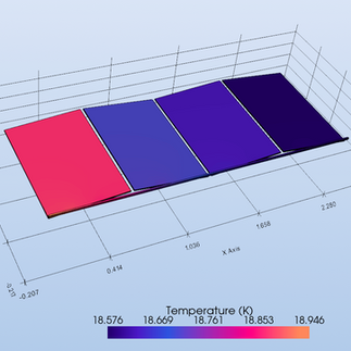
Demo 4: Black Body Radiation

This example models a very simplified geometrical representation of space radiator panels. Its not a structurally realistic model by any means, just something to show off the black body radiation boundary condition.

A total power of 1000W is applied to a connecting structure with the radiator panels connected that bar. The radiator panels are radiation with an emissivity of 0.85 to 5K ambient.

The radiator panel geometry

The model mesh.

The boundary condition assignment

The boundary temperature.

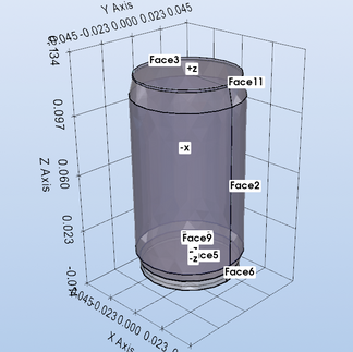
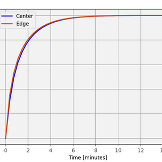
Demo 5: Transient Heat Conduction

This demo shows the working of the transient solver. It features a simple Soda can with a temperature of 5 degrees Celcius and an aluminium shell exposed to 30 degree weather. Usually, heating involves a lot of air flow and irradiance. To simplify this model I use a fixed boundary heat flux of 22W/m²K to ambient of 30 degrees and then execute a transient simulation. Two sample points are used to measure the temperature over time:

The selected faces for the Convection boundary condition.

The Soda can

The temperature over time.

What is ahead

The current setup already allows for a lot of different simulations. Some cases however are not yet supported and will be worked on soon.

Non-linear transient solver

The current module only has a non-linear solver or a transient solver. The non-linear solver can be combined with a transient solver to allow for transient solutions of the black-body radiation boundary condition. In general this is a specific simulation case that is not too important for most cases.

Surface losses and surface heating

The only coupling of RF heating into the thermal domain is through volumetric losses. Surface losses from the EM simulation cannot be imported yet. For the SurfaceImpedance boundary condition this is not too difficult.

The biggest obstacle is the absence of a thin-conductor boundary for the RF domain. This requires splitting of field degrees of freedom in order to allow for a dissimilar tangent electric field. The thermal solver has this DoF splitting routine implemented which was a great case to gain experience for the implementation in the RF domain!

Currently, to model losses of RF copper traces, you have to model them with a finite thickness. This will also automatically allow for volumetric heating.

Optimization in multi-physics coupling

To import heating into the thermal domain, the losses need to be computed inside the tetrahedra at so called Gauss-Quadrature points. These are fixed coordinates that allow for easy numeric integration.

The current implementation simply uses the interpolate function of the MWField class which needs to do a lookup first to see in which tetrahedron each sample point lies. for irregular grids this is required. For Gauss Quadrature points it strictly speaking isn't because you generate the points per tetrahedron, thus you already know in which they are. So that part can be accelerated.

For more performance, the installation of the optional Rust acceleration module EMerge-IRON is advised (www.github.com/FennisRobert/EMerge-IRON )

Periodic boundary condition

The periodic boundary condition is currently not implemented in the thermal domain. For periodic structures they may be desirable in the future. In general however, leaving the boundary conditions empty will have similar effects.

Post processing variables

Currently, the temperature, heat flux and if applicable, time stamp of the simulation are exported. There can be more exportable quantities here. Additionally, the transient simulator cannot be animated yet.

Improved non-linear solver

Currently the non-linear solver uses Anderson acceleration to offer improved performance over the otherwise naive fixed-point iterative solver. By implementing an explicit gradient solution, a Newton-Raphson method could be implemented. This involve more complex matrix assembly in order to explicitly solve for the derivative of the temperature.

Two-way solver with temperature dependence

A true multi-physics solver would be able to take into account the temperature in cases where materials would have temperature dependent electromagnetic properties. This would involve a two-way solver that iterates between the EM solver and thermal solver to find the steady-state solution.

This is currently not implemented but can, in theory, be implemented manually by simply making the dielectric properties a fucntion of coordinates and using the .interpolate() function of the heat-conduction solution as input of that function. The solve loop would have to be written manually as well.

This will eventually be included in a next version as well.

Conclusion

The first important building blocks of a multi-physics solver have been implemented. While not finished, a lot of interesting use cases can already be simulated with reasonable accuracy.

In general it must be noted that thermal simulation depend a lot on difficult to predict quantities, primarily the thermal constriction resistance. When a PCB is screwed against an aluminium block, air gaps may form, especially when there is a lot of force applied which might curve the PCB slightly. These thermal resistances can be modeled with a ThermalContact boundary condition but the exact value for the heat transfer coefficient have to be estimated.

Because these can be difficult to predict beforehand, one may wonder how important the details of a temperature dependent solver are. In some cases, thermal expansion can detune filters. This would require the addition of a mechanical solver as well but this is not on the near horizon. For now, the thermal solver is most useful to estimate temperature profiles.